Linear Algebra in Data Science: Understanding the Basics

Welcome to the fascinating world of data science, where numbers tell stories, patterns reveal insights, and equations solve problems. At the heart of this world lies a powerful mathematical tool: linear algebra. It’s the language through which data speaks. In this blog, we’ll explore the fundamental concepts of linear algebra – vectors, matrices, and scalars – and understand their basic operations. Whether you’re a budding data scientist or just curious about how data works, this journey through linear algebra will equip you with essential insights.

Understanding Vectors, Matrices, and Scalars

Vectors: In data science, vectors are like arrows pointing in a specific direction and length. They represent data points. For instance, a vector could represent a person’s height and weight as [5.5 ft, 130 lbs]. In technical terms, it’s an array of numbers.

Matrices: Think of matrices as Excel spreadsheets. They are arrays of numbers arranged in rows and columns. Each row or column can represent different variables or data points. For example, a matrix might represent the heights and weights of multiple people.

Scalars: Scalars are the simplest form of linear algebra. They are just single numbers, like 3 or -5. In the context of vectors and matrices, scalars stretch or shrink them.

Basic Operations in Linear Algebra

Vector Addition: Adding vectors is like walking in steps. If one vector represents 5 steps east, and another represents 3 steps north, their sum is a vector that represents walking 5 steps east and then 3 steps north.

Scalar Multiplication: This operation involves multiplying a vector by a scalar. It’s like stretching or shrinking the vector. If you have a vector [2, 3] and multiply it by a scalar 2, the vector becomes [4, 6].

Matrix Multiplication: This is where things get interesting. Matrix multiplication combines two matrices to form a new matrix. It’s not just multiplying each element; it’s a series of dot products between rows and columns. For example, multiplying a 2×3 matrix with a 3×2 matrix results in a 2×2 matrix.

Real-life Example: Representing Data Sets

Imagine you run a small bookstore. You keep track of the number of different genres of books sold each day. This data can be represented as a matrix, where each row is a day, and each column is a genre. By applying linear algebra operations, you can analyze trends, like which genre sells best on weekends or how sales have grown over time.

The Power of Linear Algebra in Data Manipulation

Data manipulation involves changing or adjusting data to make it more organized and easier to read. In data science, linear algebra is like the toolbox that makes this possible. It allows us to perform operations that can rearrange, categorize, and even simplify our data.

Linear Transformations: The Heart of Data Transformation

A linear transformation is a way of moving and scaling data while keeping the grid lines parallel and evenly spaced. It’s like reshaping dough – the dough itself doesn’t change, but its form does. In mathematical terms, linear transformations are functions that take vectors as inputs and produce vectors as outputs, following two main rules: lines remain lines, and the origin stays fixed.

These transformations are crucial in data science for several reasons:

• They help in rotating, scaling, and translating data points.
• They are fundamental to algorithms for machine learning and data modelling.
• They maintain the structure of the data while allowing for its manipulation.

Matrix Multiplication: A Key Tool in Data Transformation

Matrix multiplication is not just a mathematical operation; it’s a way to apply linear transformations to data. When we multiply a matrix (representing our data) by another matrix (representing the transformation), we effectively transform the entire dataset.

Example: Scaling Data with Matrix Multiplication

Let’s consider a simple example. Suppose you have a dataset representing sales figures for different products over various months. By using matrix multiplication, you can scale this data to adjust for seasonal effects or inflation. For instance, multiplying your sales data matrix by a scaling matrix can normalise your data, making year-to-year comparisons more meaningful.

Understanding Systems of Linear Equations in Data Science

A system of linear equations is a collection of linear equations involving the same set of variables. In data science, these systems can represent a range of problems, from optimising resource allocation to predicting future trends. Solving these systems helps us find values for our variables that satisfy all equations simultaneously.

Methods of Solving Linear Equations

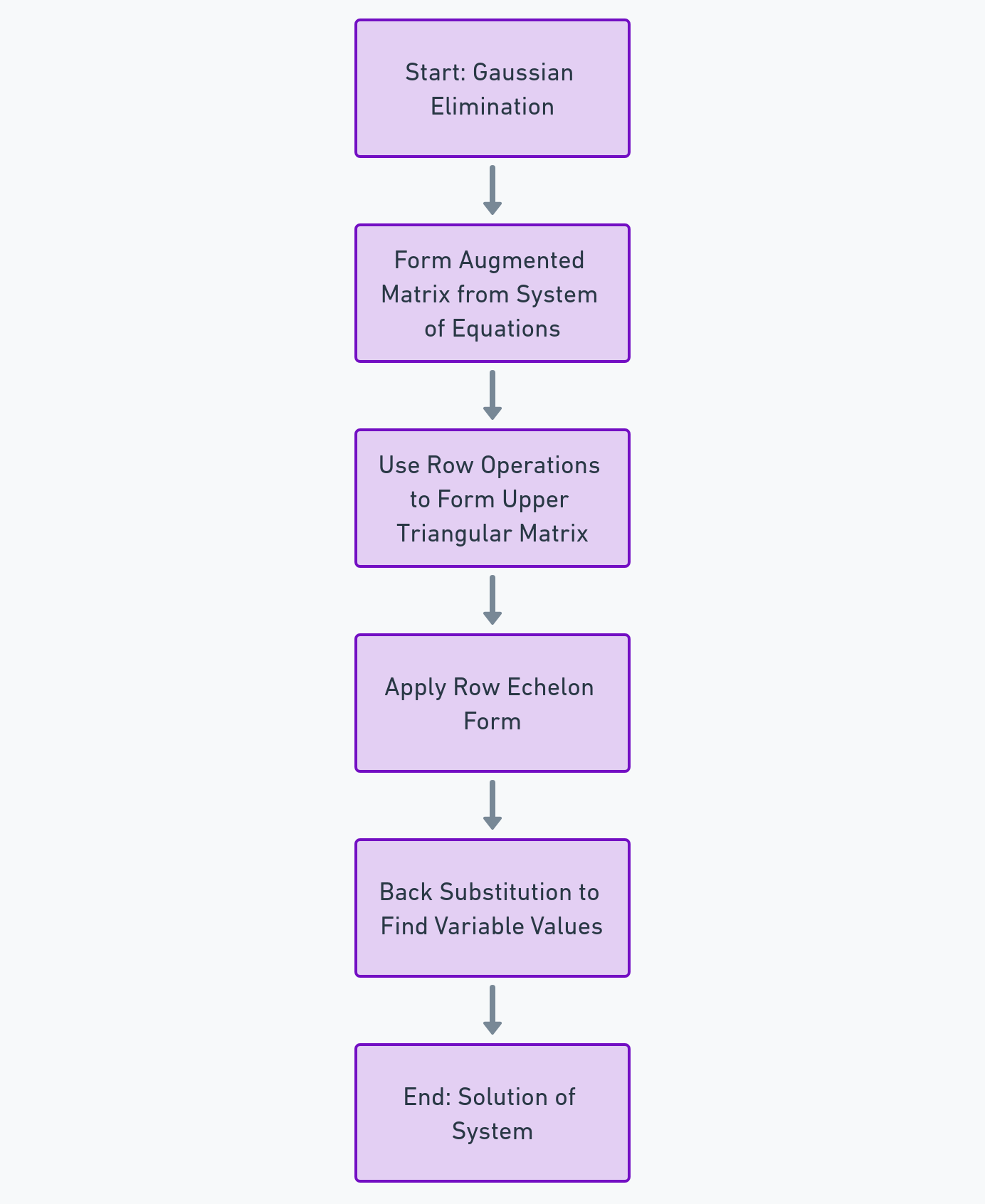
1. Gaussian Elimination: This method involves three steps – swapping, multiplying, and adding rows – to transform the matrix into a row-echelon form. From there, we can easily solve for the variables. It’s like untangling a web, strand by strand until everything is clear.
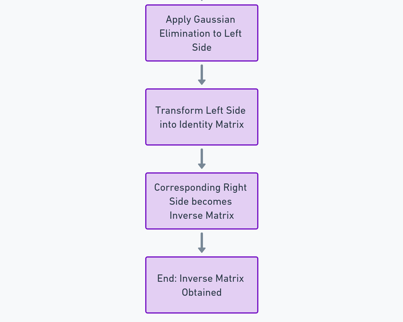
2. Matrix Inversion: Another method is using matrix inversion. This is akin to finding a key that unlocks a coded message. By multiplying the inverse of a matrix by a vector, we can find the solution to our system of equations.

Example: Predicting Sales Using Linear Equations

Imagine you’re a data scientist at a retail company, and you want to predict future sales based on past performance. You have data on sales, advertising spend, and market trends over the past year. By setting up a system of linear equations, each representing a different aspect of your sales data, you can use either Gaussian elimination or matrix inversion to solve these equations. The solution will give you insights into how different factors are influencing sales, allowing you to make informed predictions about future trends.

Understanding Eigenvalues and Eigenvectors

Eigenvalues: Imagine a transformation that changes the size of an object but not its direction. The factor by which the size changes is the eigenvalue. In mathematical terms, an eigenvalue is a scalar that indicates how much a transformation changes the size of a vector.

Eigenvectors: These are vectors that don’t change their direction during a transformation. They might get stretched or squished (by the eigenvalue), but their direction remains constant. In data science, eigenvectors help us understand the directions of maximum variance in the data.

The Significance of Eigenvalues and Eigenvectors in Data Science

Eigenvalues and eigenvectors are crucial in understanding and simplifying complex data sets. They help in identifying the underlying structure of the data, revealing patterns that are not immediately obvious. This is particularly useful in high-dimensional data, where traditional analysis methods might fall short.

Principal Component Analysis (PCA): A Practical Application

PCA is a technique used for dimensionality reduction. It transforms a large set of variables into a smaller one that still contains most of the information in the large set. The process involves finding the eigenvalues and eigenvectors of a data set, which represent the “principal components” – the directions of maximum variance.

Example: Simplifying Data Sets with PCA

Let’s consider a real-world example. Imagine you’re analyzing a dataset containing hundreds of variables on customer behavior. Analyzing this dataset in its entirety is challenging due to its size. By applying PCA, you can reduce these variables to a smaller number that still captures the essence of customer behavior. This is achieved by finding the eigenvectors (principal components) and their corresponding eigenvalues, which tell us how much of the data’s variance is captured by each component. This simplification makes it easier to perform further analysis, like clustering or predictive modeling.

Eigenvalues, Eigenvectors, and Beyond

The beauty of eigenvalues and eigenvectors lies in their ability to distill complexity into simplicity. They provide a way to look at data from a different perspective, one that highlights the most significant aspects while reducing noise and redundancy.

What is Singular Value Decomposition (SVD)?

SVD is a technique that decomposes a matrix into three other matrices, known as the singular matrices. These matrices represent different aspects of the original data: its direction, scaling, and another direction. The beauty of SVD lies in its ability to distill complex, high-dimensional data into its most meaningful components.

The Role of SVD in Data Science

In data science, SVD is used for:

• Dimensionality Reduction: Similar to PCA, SVD reduces the number of variables in a dataset while retaining its essential characteristics.
• Noise Reduction: SVD helps in filtering out noise or unnecessary information from data.
• Feature Extraction: It extracts the most important features from a dataset, which can be crucial for machine learning models.

Application of SVD in Recommender Systems

One of the most exciting applications of SVD is in the development of recommender systems. These systems analyze patterns in user behaviour to recommend products, movies, or music. SVD helps in understanding these patterns by breaking down user-item matrices into simpler matrices that represent user preferences and item characteristics.

Example: Building a Basic Movie Recommender System Using SVD

Imagine you’re tasked with creating a movie recommendation system for a streaming platform. You have a dataset containing user ratings for various movies. Here’s how you could use SVD:

1. Data Preparation: Organise the data into a user-movie rating matrix, where each row represents a user and each column represents a movie.
2. Applying SVD: Perform SVD on this matrix. This will decompose your matrix into three matrices, capturing the essence of users’ preferences and movies’ features.
3. Making Recommendations: Use these matrices to predict how a user would rate movies they haven’t seen yet. Recommend movies with the highest predicted ratings.

SVD in Image Compression

Another application of SVD is in image compression. By decomposing an image into singular matrices, SVD enables us to approximate the image using fewer data points, thereby compressing it without significant loss of quality.

Linear Algebra in Machine Learning Algorithms

Machine learning algorithms are fundamentally about finding patterns in data. Linear algebra provides the framework for organizing and manipulating large datasets, making it possible to apply these algorithms efficiently. Whether it’s support vector machines, neural networks, or clustering algorithms, linear algebra’s matrices and vectors are at the core of these computations.

Linear Regression from a Linear Algebra Perspective

Linear regression, one of the simplest yet powerful machine learning algorithms, is a perfect example of linear algebra in action. It involves finding the best linear relationship between the independent and dependent variables. In linear algebra terms, this translates to finding the best-fit line through a multidimensional space of data points, which is achieved by minimizing the distance between the data points and the line.

Logistic Regression: Beyond Linear Boundaries

While linear regression is suited for continuous output, logistic regression is used for classification problems. It predicts the probability of a data point belonging to a particular class. Linear algebra plays a role in calculating these probabilities and in determining the decision boundary, a concept that separates different classes in the dataset.

Example: Implementing Linear Regression on a Dataset

Let’s put theory into practice by implementing linear regression on a dataset. Suppose we have a dataset of housing prices, with features like size, number of bedrooms, and age of the house. Our goal is to predict the price of a house based on these features.

1. Data Representation: We represent our features and target variable (house prices) as matrices and vectors.
2. Model Training: Using linear algebra, we calculate the coefficients (weights) that provide the best prediction of house prices. This involves solving a system of linear equations or using optimization techniques like gradient descent.
3. Prediction: With our model trained, we can now predict the price of a house given its features, using the weights we’ve calculated.

Conclusion

Linear algebra is not just a set of mathematical concepts; it’s the foundation upon which machine learning models are built. Understanding its principles and applications is crucial for anyone venturing into machine learning. As we continue to explore the applications of linear algebra in data science, its significance becomes ever more apparent.